前言
本文是南京大学李樾、谭添老师的《软件分析》课程的笔记。内容来自课程ppt以及课程讲解。
课程主页:Static Program Analysis | Tai-e (pascal-lab.net)
授课视频:视频南京大学《软件分析》课程01(Introduction)_哔哩哔哩_bilibili
课程实验repo:pascal-lab/Tai-e-assignments: Tai-e assignments for static program analysis (github.com)
Contents
- Iterative Algorithm, Another View
- Partial Order
- Upper and Lower Bounds
- Lattice, Semilattice, Complete and Product Lattice
- Data Flow Analysis Framework via Lattice
- Monotonicity and Fixed Point Theorem
- Relate Iterative Algorithm to Fixed Point Theorem
- May/Must Analysis, A Lattice View
- MOP and Distributivity
- Constant Propagation
- Worklist Algorithm
Review The Questions We Have Seen Before
The iterative algorithm (or the IN/OUT equation system) produces a solution to a data flow analysis
- Is the algorithm guaranteed to terminate or reach the fixed point, or does it always have a solution?
- If so, is there only one solution or only one fixed point? If more than one, is our solution the best one (most precise)?
- When will the algorithm reach the fixed point, or when can we get the solution?
Now what we have just seen is the property (fixed point theorem) for the function on a lattice. We cannot say our iterative algorithm also has that property unless we can relate the algorithm to the fixed point theorem, if possible
Relate Iterative Algorithm to Fixed-Point Theorem
- → $(\bot, \bot …, \bot)$
- iter 1 → $(v_1^1, v_2^1, …, v_k^1)$
- iter 2 → $(v_1^2, v_2^2, …, v_k^2)$
- …
- iter i → $(v_1^i, v_2^i, …, v_k^i)$
- iter i+1 → $(v_1^i, v_2^i, …, v_k^i)$
Given a complete lattice (L, ⊑), if
(1) f: L → L is monotonic and (2) L is finite,
then the least fixed point of f can be found by iterating $f(⊥), f(f(⊥)), …, f^k(⊥)$ until a fixed point is reached the greatest fixed point of f can be found by iterating $f( ), f(f( )), …, f^k( )$ until a fixed point is reached
If a product lattice $L^k$ is a product of complete (and finite) lattices, i.e., (L, L, …, L), then $L^k$ is also complete (and finite)
In each iteration, it is equivalent to think that we apply function F which consists of (1) transfer function fi : L → L for every node (2) join/meet function ⊔/⊓: L×L → L for control-flow confluence
Now the remaining issue is to prove that function F is monotonic
Prove Function F is Monotonic
In each iteration, it is equivalent to think that we apply function F which consists of
transfer function fi : L → L for every node
Gen/Kill function is monotonic
join/meet function ⊔/⊓: L×L → L for control-flow confluence
Actually the binary operator is a basic case of L × L ×… × L, we want show that ⊔ is monotonic
Proof.
∀x, y, z ∈ L, x ⊑ y, we want to prove x ⊔ z ⊑ y ⊔ z
by the definition of ⊔, y ⊑ y ⊔ z
by transitivity of ⊑, x ⊑ y ⊔ z
thus y ⊔ z is an upper bound for x, and also for z (by ⊔’s definition) as x ⊔ z is the least upper bound of x and z
thus x ⊔ z ⊑ y ⊔ z
Thus the fixed point theorem applies to the iterative algorithm for data flow analysis.
When Will the Algorithm Reach the Fixed Point?
The height of a lattice h is the length of the longest path from Top to Bottom in the lattice.
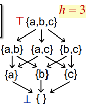
The maximum iterations i needed to reach the fixed point
In each iteration, assume only one step in the lattice (upwards or downwards) is made in one node (e.g., one 0->1 in RD)
Assume the lattice height is h and the number of nodes in CFG is k
We need at most i = h*k iterations
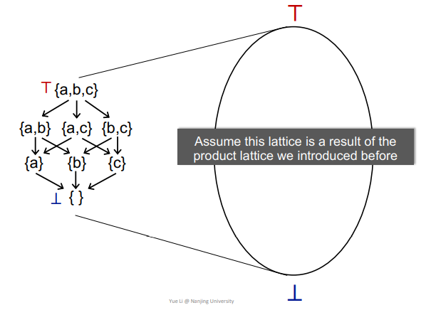
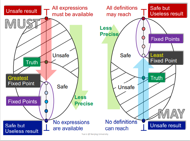
May and Must Analyses, a Lattice View
MOP and Distributivity
How Precise Is Our Solution?
Meet-Over-All-Paths Solution(MOP)
$P = Entry \rightarrow S_1 \rightarrow S_2 \rightarrow \dots \rightarrow S_i$
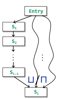
Transfer function $FP$ for a path P (from Entry to $S_i$ ) is a composition of transfer functions for all statements on that path: $f{S1}$, $f{S2}$, …, $f{S_{i-1}}$
$MOP[S_i]=⊔/⊓ F_P(OUT[Entry])$
MOP computes the data-flow values at the end of each path and apply join / meet operator to these values to find their lub / glb
Some paths may be not executable -> not fully precise
Unbounded, and not enumerable -> impratical
Ours(Iterative Alorithm) vs. MOP
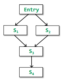
$IN[S4]=f{s3}(f{s1}(OUT[Entry])⊔f{s_2}(OUT[Entry]))$
$MOP[S4]=f{s3}(f{s1}(OUT[Entry]))⊔f{s3}(f{s_2}(OUT[Entry]))$
Ours = F(x⊔y), MOP = F(x) ⊔ F(y)
By definition of lub ⊔, we have
x ⊑ x ⊔ y and y ⊑ x ⊔ y
As transfer function F is monotonic, we have
F(x) ⊑ F(x ⊔ y) and F(y) ⊑ F(x ⊔ y)
That means F(x ⊔ y) is an upper bound of F(x) and F(y)
As F(x) ⊔ F(y) is the lub of F(x) and F(y), we have
F(x) ⊔ F(y) ⊑ F(x ⊔ y)
MOP ⊑ Ours
(Ours is less precise than MOP)
When F is distributive, i.e., F(x ⊔ y) = F(x) ⊔ F(y), MOP=Ours(Ours is as precise as MOP)
Bit-vector or Gen/Kill problems (set union /intersection for join/meet) are distributive, but some analyses are not distributie.
Constant Propagation
Given a variable x at program point p, determine whether x is guaranteed to hold a constant value at p.
The OUT of each node in CFG, includes a set of pairs (x, v) where x is a variable and v is the value held by x after that node
A data flow analysis framework (D, L, F) consists of:
- D: a direction of data flow: forwards or backwards
- L: a lattice including domain of the values V and a meet ⊓ or join ⊔ operator
- F: a family of transfer functions from V to V
Lattice
Domain of the values V
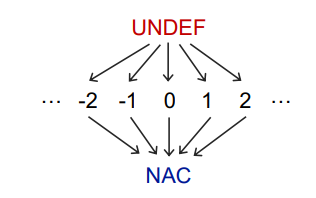
Meet Operator ⊓
- NAC ⊓ v = NAC
- UNDEF ⊓ v = v
- c ⊓ c = c
- c1 ⊓ c2 = NAC
Transfer Function
Given a statement s: x = …, we define its transfer function F as
$F:OUT[s]=gen \cup (IN[s] - {(x,_)})$
(we use val(x) to denote the lattice value that variable x holds)
- s: x = c // c is a constant gen = {x,c}
- s: x = y gen = {(x, val(y))}
- s: x = y op z gen = {(x,f(y,z))}
f{y,z} =
- val(y) op val(z) // if val(y) and val(z) are constants
- NAC // if val(y) or val(z) is NAC
- UNDEF // otherwise
(if s is not an assignment statement, F is the identity function)
Nondistributivity
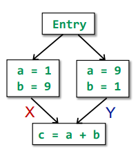
F(X ⊓ Y) = {(a,NAC), (b,NAC), (c,NAC)}
F(x) ⊓ F(Y) = {(a, NAC), (b, NAC), (c,10)}
F(X ⊓ Y) ≠ F(x) ⊓ F(Y) and F(X ⊓ Y) ⊑ F(x) ⊓ F(Y)
Worklist Algorithm, an optimization of Iterative Algorithm
Review Iterative Algorithm for May&Forward Analysis
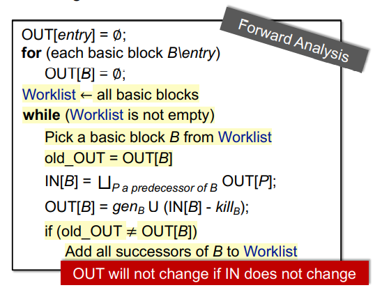
INPUT: CFG($kill_B$ and $gen_B$ computed for each basic block B)
OUTPUT: $IN[B]$ and$OUT[B]$ for each basic block B
METHOD: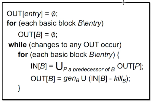
WorkList Algorithm
