前言
本文是南京大学李樾、谭添老师的《软件分析》课程的笔记。内容来自课程ppt以及课程讲解。
课程主页:Static Program Analysis | Tai-e (pascal-lab.net)
授课视频:视频南京大学《软件分析》课程01(Introduction)_哔哩哔哩_bilibili
课程实验repo:pascal-lab/Tai-e-assignments: Tai-e assignments for static program analysis (github.com)
Contents
- Iterative Algorithm, Another View
- Partial Order
- Upper and Lower Bounds
- Lattice, Semilattice, Complete and Product Lattice
- Data Flow Analysis Framework via Lattice
- Monotonicity and Fixed Point Theorem
- Relate Iterative Algorithm to Fixed Point Theorem
- May/Must Analysis, A Lattice View
- MOP and Distributivity
- Constant Propagation
- Worklist Algorithm
Iterative Algorithm, Anthor View
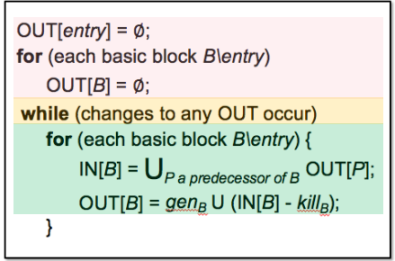
Given a CFG (program) with k nodes, the iterative algorithm updates OUT[n] for every node n in each iteration.
Assume the domain of the values in data flow analysis is V, then we can define a k-tuple
$(OUT[n_1], OUT[n_2], …, OUT[n_k])$
as an element of set $(V_1 × V_2 × … × V_3)$denoted as $V^k$ , to hold the values of the analysis after each iteration
Each iteration can be considered as taking an action to map an element of Vk to a new element of Vk , through applying the transfer functions and control-flow handing, abstracted as a function$F: V^k \rightarrow V^k$
Then the algorithm outputs a series of k-tuples iteratively until a k-tuple is the same as the last one in two consecutive iterations
Given a CFG (program) with $k$ nodes, the iterative algorithm updates $OUT[n]$ for every node n in each iteration.
Each iteration takes an action$F: V^k \rightarrow V^k$
- init → $(\bot, \bot …, \bot) = X_0$
- iter 1 → $(v_1^1, v_2^1, …, v_k^1) = X_1 = F(X_0)$
- iter 2 → $(v_1^2, v_2^2, …, v_k^2) = X_2 = F(X_1)$
- …
- iter i → $(v1^i, v_2^i, …, v_k^i) = X_i = F(X{i-1})\because Xi=X{i+1}$
- iter i+1 → $(v1^i, v_2^i, …, v_k^i) = X{i+1} = F(X{i})\therefore X_i=X{i+1}=F(X_i)$
X is a fied of function F if $X=F(X)$
The iterative algorithm reaches a fixed point
The iterative algorithm (or the IN/OUT equation system) produces a solution to a data flow analysis
- Is the algorithm guaranteed to terminate or reach the fixed point, or does it always have a solution?
- If so, is there only one solution or only one fixed point? If more than one, is our solution the best one (most precise)?
- When will the algorithm reach the fixed point, or when can we get the solution?
Partial Order
Definition
We define poset as a pair (P, ⊑) where ⊑ is a binary relation that defines a partial ordering over P, and ⊑ has the following properties:
- ∀x ∈ P, x ⊑ x (Reflexivity)
- ∀x, y ∈ P, x ⊑ y ∧ y ⊑ x ⟹ x = y (Antisymmetry)
- ∀x, y, z ∈ P, x ⊑ y ∧ y ⊑ z ⟹ x ⊑ z (Transitivity)
Example
Example 1
Is (S, ⊑) a poset where S is a set of integers and ⊑ represents ≤ (less than or equal to)?
- Reflexivity 1 ≤ 1, 2 ≤ 2 √
- Antisymmetry x ≤ y ∧ y ≤ x then x = y √
- Transitivity 1 ≤ 2 ∧ 2 ≤ 3 then 1 ≤ 3 √
Example 2
Is (S, ⊑) a poset where S is a set of integers and ⊑ represents < (less than)?
(1) Reflexivity 1 < 1, 2< 2 ×
Example 3
Is (S, ⊑) a poset where S is a set of English words and ⊑ represents the substring relation, i.e., s1 ⊑ s2 means s1 is a substring of s2?
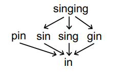
- Reflexivity √
- Antisymmetry √
- Transitivity √
Example 4
Is (S, ⊑) a poset where S is the power set of set {a,b,c} and ⊑ represents ⊆ (subset)?
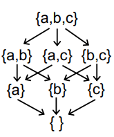
- Reflexivity √
- Antisymmetry √
- Transitivity √
Upper and Lower Bounds
Given a poset (P, ⊑) and its subset S that S ⊆ P, we say that u ∈ P is an upper bound of S, if ∀x ∈ S, x ⊑ u. Similarly, l ∈ P is an lower bound of S, if ∀x ∈ S, l ⊑ x.
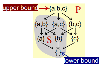
We define the least upper bound (lub or join) of S, written ⊔S, if for every upper bound of S, say u, ⊔S ⊑ u. Similarly, We define the greatest lower bound (glb, or meet) of S, written ⊓S, if for every lower bound of S, say l, l ⊑ ⊓S.
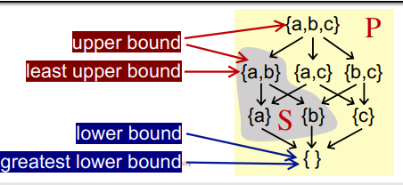
Usually, if S contains only two elements a and b (S = {a, b}), then ⊔S can be written a ⊔ b (the join of a and b) ⊓S can be written a ⊓ b (the meet of a and b)
Some Properties
Not every poset has lub or glb
But if a poset has lub or glb, it will be unique
Proof:
assume g1 and g2 are both glbs of poset P
according to the definition of glb
g1 ⊑ (g2 = ⊓P) and g2 ⊑ (g1 = ⊓P)
by the antisymmetry of partial order ⊑
g1 = g2
Lattice, Semilattice, Complete and Product Lattice
Lattice
Given a poset (P, ⊑), ∀a, b ∈ P, if a ⊔ b and a ⊓ b exist, then (P, ⊑) is called a lattice
A poset is a lattice if every pair of its elements has a least upper bound and a greatest lower bound
Example
Example 1
Is (S, ⊑) a lattice where S is a set of integers and ⊑ represents ≤ (less than or equal to)?
The ⊔ operator means “max” and ⊓ operator means “min” √
Example 2
s (S, ⊑) a lattice where S is a set of English words and ⊑ represents the substring relation, i.e., s1 ⊑ s2 means s1 is a substring of s2?

pin ⊔ sin = ? ×
Example 3
Is (S, ⊑) a lattice where S is the power set of set {a,b,c} and ⊑ represents ⊆ (subset)?

The ⊔ operator means ∪ and ⊓ operator means ∩ √
Semilattice
Given a poset (P, ⊑), ∀a, b ∈ P, if only a ⊔ b exists, then (P, ⊑) is called a join semilattice if only a ⊓ b exists, then (P, ⊑) is called a meet semilattice
Complete Lattice
Given a lattice (P, ⊑), for arbitrary subset S of P, if ⊔S and ⊓S exist, then (P, ⊑) is called a complete lattice
All subsets of a lattice have a least upper bound and a greatest lower bound
Example
Example 1
Is (S, ⊑) a complete lattice where S is a set of integers and ⊑ represents ≤ (less than or equal to)?
For a subset $S^+$ including all positive integers, it has no ⊔$S^+$ (+∞)
Example 2
Is (S, ⊑) a complete lattice where S is the power set of set {a,b,c} and ⊑ represents ⊆ (subset)?

√
Note: the definition of bounds implies that the bounds are not necessarily in the subsets (but they must be in the lattice)
Every complete lattice (P, ⊑) has a greatest element = ⊔P called top and a least element ⊥ = ⊓P called bottom
Every finite lattice (P is finite) is a complete lattice
Product Lattice
Given lattices L1 = (P1, $⊑_1$), L2 = (P2, $⊑_2$), …, Ln = (Pn, $⊑_n$), if for all i, (Pi , $⊑_i$ ) has $⊔_i$ (least upper bound) and $⊓_i$ (greatest lower bound), then we can have a product lattice $L^n = (P, ⊑)$ that is defined by:
- $P = P_1 × … × P_n$
- $(x_1,…,x_n)⊑(y_1,…,y_n)\Leftrightarrow(x_1⊑y_1)∧…∧(x_n⊑y_n)$
- $(x_1,…,x_n)⊔(y_1,…,y_n)=(x_1⊔_1y_1,…,x_n⊔_ny_n)$
$(x_1,…,x_n)⊓(y_1,…,y_n)=(x_1⊓ _1y_1,…,x_n⊓ _ny_n)$
A product lattice is a lattice
- If a product lattice L is a product of complete lattices, then L is also complete
Data Flow Analysis Framework via Lattice
A data flow analysis framework (D, L, F) consists of:
- D: a direction of data flow: forwards or backwards
- L: a lattice including domain of the values V and a meet ⊓ or join ⊔ operator
- F: a family of transfer functions from V to V
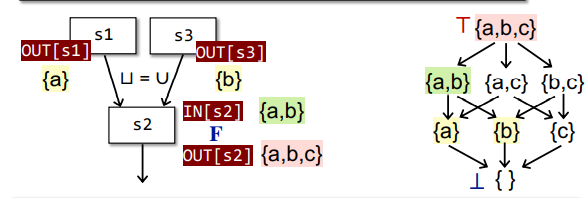
Data flow analysis can be seen as iteratively applying transfer functions and meet/join operations on the values of a lattice
Monotonicity and Fixed Point Theorem
Monotonicity
A function f: L → L (L is a lattice) is monotonic if ∀x, y ∈ L, x ⊑ y ⟹ f(x) ⊑ f(y)
Fixed-Point Theorem
Given a complete lattice (L, ⊑), if
(1) f: L → L is monotonic and (2) L is finite,
then the least fixed point of f can be found by iterating $f(⊥), f(f(⊥)), …, f^k(⊥)$ until a fixed point is reached the greatest fixed point of f can be found by iterating $f( ), f(f( )), …, f^k( )$ until a fixed point is reached
Prove: Existence of fixed point
Proof:
By the definition of ⊥ and f: L → L, we have $⊥ ⊑ f(⊥)$
As f is monotonic, we have $f(⊥) ⊑ f(f(⊥)) = f^2(⊥)$
By repeatedly applying f, we have an ascending chain $⊥ ⊑ f(⊥) ⊑ f^2(⊥) ⊑ … ⊑ f^i (⊥)$
As L is finite (its height is H), the values are bounded among $⊥ , f(⊥) , f^2(⊥) … f^H(⊥)$
When i > H, by pigeonhole principle, there exists k and j that $f^k(⊥) = f^j (⊥) (assume k < j ≤ H+1)$
Further as fk(⊥) ⊑ … ⊑ fj (⊥), we have $f^{Fix} = f^k(⊥) = f^{k+1}(⊥) = f^j (⊥)$
Thus, the fixed point exists.
Prove: Least Fixed Point
Proof:
Assume we have another fixed point x, i.e., x = f(x)
By the definition of ⊥, we have ⊥ ⊑ x
Induction begins:
As f is monotonic, we have f(⊥) ⊑ f(x)
Assume $f^i (⊥) ⊑ f^i (x)$, as f is monotonic, we have $f^{i+1}(⊥) ⊑ f{i+1}(x)$
Thus by induction, we have $f^i (⊥) ⊑ f^i (x)$
Thus $f^i (⊥) ⊑ f^i (x) = x$, then we have $f^{Fix} = f^k(⊥) ⊑ x$
Thus the fixed point is the least
Now what we have just seen is the property (fixed point theorem) for the function on a lattice. We cannot say our iterative algorithm also has that property unless we can relate the algorithm to the fixed point theorem, if possible