前言

本文是南京大学李樾、谭添老师的《软件分析》课程的笔记。内容来自课程ppt以及课程讲解。

课程主页：Static Program Analysis | Tai-e (pascal-lab.net)

授课视频：视频南京大学《软件分析》课程01（Introduction）_哔哩哔哩_bilibili

课程实验repo：pascal-lab/Tai-e-assignments: Tai-e assignments for static program analysis (github.com)

Overview of Data Flow Analysis
Preliminaries of Data Flow Analysis
Reaching Definitions Analysis
Live Variables Analysis
Available Expressions Analysis

Overview of Data Flow Analysis

Data Flow Analysis -> How Data flows on CFG?

-> How application-specfific Data Flows through the Nodes(BBs/statements) and Edges(control flows) of CFG(a program)?

application-specfific Data: Abstraction, + - 0 $\top$ $\bot$
Flows: Safe-approximation. For most stactic analyses are “may analysis”
- may analysis: outputs information that may be true (over-approximation)
- must analysis: outputs information that must be true (under-approximation)
- Over- and under-approximations are both for safety of analysis
Nodes: Transfer function, e.g. (+) + (+) = (+)
Edges: Control-flow handing: Union the sign at merges

different data-flow analysis applications have

different data abstraction and

different flow safe-approximation strategies, i.e.,

different transfer functions and control-flow handlings

Preliminaries of Data Flow Analysis

Input and Output States

Each execution of an IR statement transforms an input state to a new output state
The input(output) state is associated with program point before(after) the statement

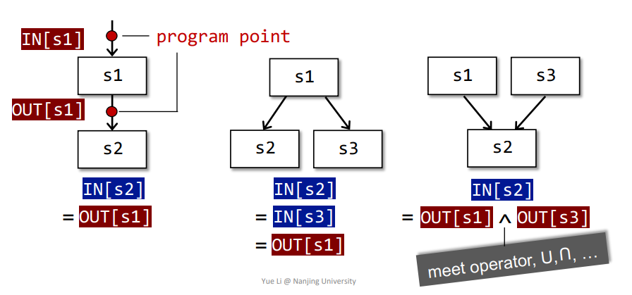
In each data-flow analysis application, we associate with every program point ==a data-flow value== that represents an ==abstraction== of the set of all possible ==program states== that can be observed for that point.

x = 10;
point  ->    x = +, y = undefine
y = -1;
point  ->    x = +, y = -
x = y;
point  ->    x = -, y = -
x = x / y;
point  ->    x = +, y = -

The set of possible data-flow values is the domain for this application(+ - 0 $\top$ $\bot$)

Data-flow analysis is to ==find a solution== to a set of ==safe-approximation directed constraints== on the IN[s]’s and OUT[s]’s, for all statements s.

constraints based on semantics of statements (transfer functions)
constraints based on the flows of control

Notations for Transfer Function’s Constraints

Forward Analysis: $OUT[s] = f_s(IN[s])$
Backward Analysis: $IN[s] = f_s(OUT[s])$

Notations for Control Flow’s Constraints

Control flow within a BB: $In[s_{i+1}] = OUT[s_i], for ~all~i = 1,2,…n-1$
Control flow among BBs:

$IN[B]=IN[s_1]$

$OUT[B]=OUT[s_n]$
- Forward:
  
  $OUT[B]=fB(IN[B]),f_B=f{sn}\circ …\circ f{s2} \circ f{s_1}$
  
  $IN[B]=\wedge P_{~a~predecessor of B}~OUT[P]$
- Backward:
  
  $IN[B]=fB(OUT[B]),f_B=f{s1}\circ f{s2} \circ …\circ f{s_n}$
  
  $OUT[B]=\wedge S_{~a~successor of B}~IN[S]$

The meet operator $\wedge$ is used to summarize the contributions from different paths at the confluence of those paths

Issues Not Covered:

Method Calls
- Intra-procedural CFG
- Will be introduced in lecture: Inter-procedural Analysis
Aliases
- Variables have no aliases
- Will be introduced in lecture: Pointer Analysis

Reaching Definitions Analysis

Reaching Definition

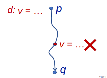
A ==definition d== at program point p ==reaches== a point q if there is a path from p to q such that ==d== is not “killed” along that path.

A definition of a variable v is a statement that assigns a value to v
Translated as: definition of variable v at program point p reaches point q if there is a path from p to q such that no new definition of v appears on that path

Reaching definitions can be used to ==detect possible undefined variables==. e.g., introduce a dummy definition for each variable v at the entry of CFG, and if th e dummy definition of v reaches a point p where v is used, then v may be used before definition (as undefined reaches v)

Understanding Reaching Definitions

Abstraction:

Data Flow Values/Facts
- The definition of all the variables in a program
- Can be represented by bit vectors
  
  e.g., D1, D2, D3, D4, …, D100 (100 efinitions)
  
  $\underbrace{0000…0}_{100}$
  
  Bit i from the left represents definition Di

Safe-approximation

1	D: v = x op y

This statement “generates” a definition D of variable v and “kills” all the other definitions in the program that define variable v, while leaving the remaining incoming definition unaffected.

Transfer Function

$OUT[B] = gen_B\cup(IN[B] - kill_B)$
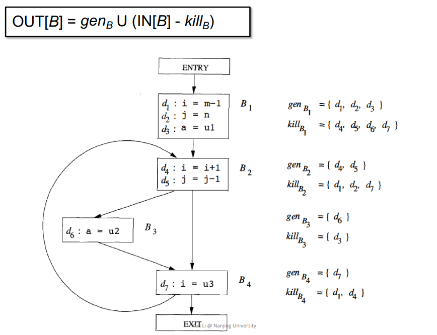
Control Flow

$IN[B]=\cup P_{~a~predecessor of B}~OUT[P]$

Algorithm of Reaching Definitions Analysis

INPUT: CFG($kill_B$ and $gen_B$ computed for each basic block B)

OUTPUT: $IN[B]$ and$OUT[B]$ for each basic block B

METHOD: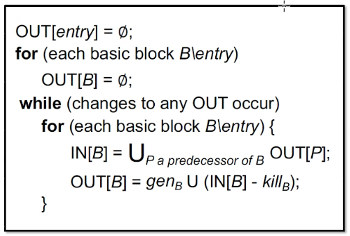

解释：

$OUT[entry]=\phi$含义:

entre没有statements 和 definition
for中each basic block $B\entry$和第一行的$OUT[entry]=\phi$ 为什么不合并？

这是经典的模板算法，并非只对Reaching Definition适用。
for中 $OUT[B]=\phi$ ?

may analysis一般为空

must analysis一般为top($\top$)
为什么这个算法最终可以停止？

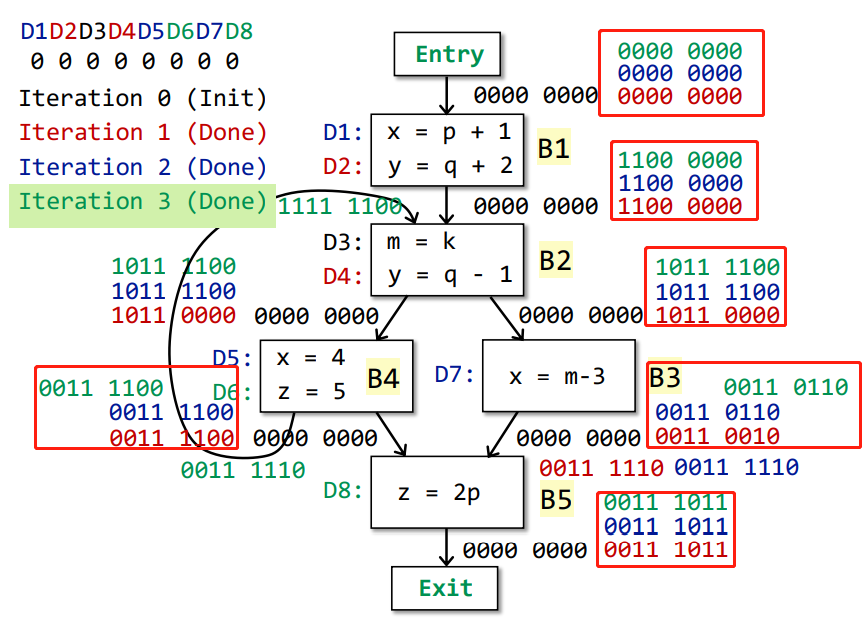
Example

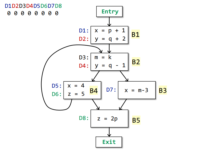
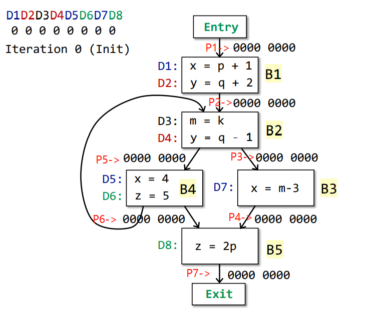
Iteration 0(Init)

	Input	gen	kill	Output
entry				0000 0000
B1				0000 0000
B2				0000 0000
B3				0000 0000
B4				0000 0000
B5				0000 0000

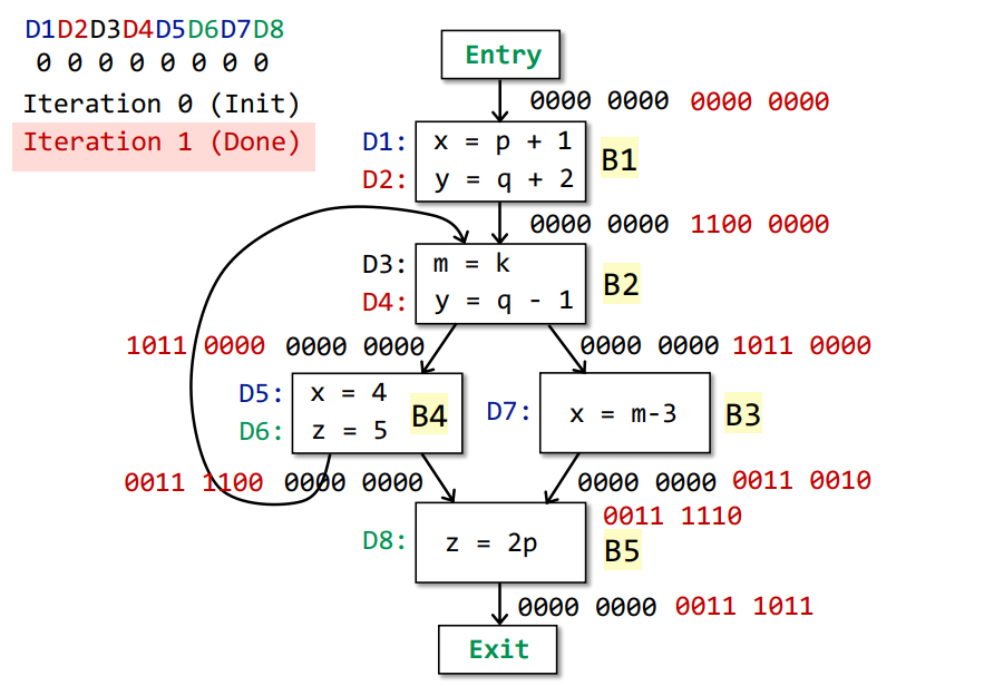
Iteration 1

	Input	gen	kill	Output
B1	0000 0000	D1 D2	D4 D5	1100 0000
B2	0000 0000(O[B4]) U 1100 0000(O[B1])	D3 D4	D2	1011 0000
B3	1011 0000	D7	D1 D5	0011 0010
B4	1011 0000	D5 D6	D1 D8	0011 1100
B5	0011 0010(O[B4]) U 0011 1100(O[B3])	D8	D6	0011 1011

Changes occur in OUT[] of B1,B2,B3,B4,B5

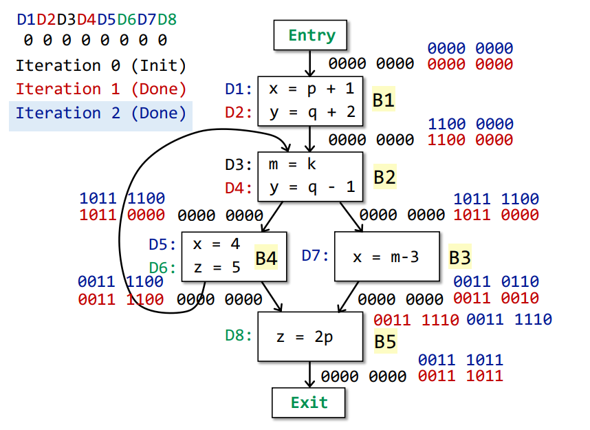
Iteration 2

	Input	gen	kill	Output
B1	0000 0000	D1 D2	D4 D5	1100 0000
B2	0011 1100(O[B4]) U 1100 0000(O[B1])	D3 D4	D2	1011 1100
B3	1011 1100	D7	D1 D5	0011 0110
B4	1011 1100	D5 D6	D1 D8	0011 1100
B5	0011 1100 U 0011 0110	D8	D6	0011 1011

Changes occur in OUT[] of B2 B3

Iteration 3

	Input	gen	kill	Output
B1	0000 0000	D1 D2	D4 D5	1100 0000
B2	0011 1100(O[B4]) U 1100 0000(O[B1])	D3 D4	D2	1011 1100
B3	1011 1100	D7	D1 D5	0011 0110
B4	1011 1100	D5 D6	D1 D8	0011 1100
B5	0011 1100 U 0011 0110	D8	D6	0011 1011

No changes occur in any OUT[]. We get the final analysis result.

Why this iterative can finally algorithm stop?

$OUT[S] = gen_S U (IN[S] - kill_S)$;

$gen_S$ and $kill_S$ remain unchanged
When more facts flow in $IN[S]$, the “more facts” either
- is killed, or
- flows to $OUTS$
When a fact is added to $OUT[S]$, through either $gen_S$, or $survivor_S$ , it stays there forever
Thus $OUT[S]$ never shrinks(e.g., 0 -> 1, or 1 -> 1)
As the set of facts is finite (e.g., all definitions in the program), there must exist a pass of iteration during which nothing is added to any OUT, and then the algorithm terminates

Safe to terminate by this condition?

IN’s will not change if OUT’s do not change
OUT’s will not change if IN’s do not change
Reach a fixed point. Also related with monotonicity(next lectures)

Write the code, Change the world

南大《软件分析》03.Data Flow Analysis - Applications I

前言

Contents